As I have said before, this course is in R- and trying to perform all the tasks in python is proving to be an interesting challenge. I want to document the new and interesting  things, I am learning along the way. It turns out that the way most generic way to run linear regression in R, is to use the lm function. As part of the summary results, you get a bunch of extra information like confidence intervals and p values for each of the coefficients,  adjusted R2, F statistic etc that you don’t get as part of the output-in sklearn -the most popular machine learning package in python. Digging a bit deeper, you can see why:

• scikit-learn is doing machine learning with emphasis on predictive modeling with often large and sparse data.
• statsmodels is doing “traditional” statistics and econometrics, with much stronger emphasis on parameter estimation and (statistical) testing. Its linear models, generalized linear models and discrete models have been around for several years and are verified against Stata and R – and the output parameters are almost identical to what you would get in R.

For this project; where I am trying to translate R to python; statsmodels is a better choice. Statsmodels can be used by importing statsmodels.api, or the statsmodels.formula.api and I have played around with both. Statsmodels.formula.api uses R like syntax as well, but Statsmodels.api has a very sklearn -like syntax. I have explored using linear regression in a few different kinds of datasets: (github repo)

• Climate data
• Sales data for a company
• Detecting flu epidemics via search engine query
• Analyzing Test scores
• State data including things like population, per capita income,murder rates etc

There are a lot of wonderful  blogs/tutorials on Linear Regression. Some of my favorite are:

• Linear Regression in Python- by dataschool
• Intro to Linear Regression
• Regression

What is different about Analytics edge is that that is a lot of emphasis on the intuitive understanding of the output of the regression algorithm.

So what is a linear regression model?     

This question has confused me at times because :

• y=Bo+B1X1+B2X2
• y=B0+B1(lnX1)
• y=Bo+B1X1+B2X**2   are all linear models, but they are not all linear in X !!

From  what I understand now, a regression model is linear, when it is linear in the parameters. What that means is there is only one parameter in each term of the model and each parameter is a multiplicative constant on the independent variable. So in the above example, (lnX1) is the parameter or variable, and the function is linear in that parameter. Similarly, (X**2) is the variable and the function is linear in that  variable.

Examples of non-linear models:

• y=B1.exp(-B2.X2)+K
• y=B1+(B2-B1)exp(-B3X) +K
• y= (B1X)/(B2+X) +K

A really important analysis to perform before you run any multivariate  linear regression model is to calculate the correlations between different variables -this is if you include because highly correlated variables as independent variables in your model, you would get some unintuitive an d inaccurate answers!! For example, if I run a multiple regression model to predict average global temperature using atmospheric concentrations of most of the greenhouse gases available from the Climatic Research Unit at the University of East Anglia, this is my output:

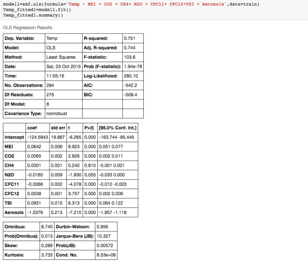
If we examine the output, and look at the coefficients and their corresponding  p_values, ie the P>|t| column, we see that  according to this model, N2O and CH4 which are both considered to be green house gases, are not significant variables!  ie the P>|t| values for those coefficients is higher that the rest.

So what is  P>|t|?                                                                                                                                           P >|t| is  probability that the coefficient for that variable is Zero, given the data used to build the model. The smaller this probability, the less likely the coefficient is actually Zero. We want independent variables with very small values for this. Note that if the coefficient of a variable is almost Zero, that variable is not helping to predict the dependent variable.

Furthermore, the coefficient of N2O is negative, implying that the global temperature is inversely proportional to the atmospheric concentration of N2O. This is contrary to what we know!  So what is going on?

It becomes clear when  we examine the correlations between the different variables:

We can see that there is  a really high correlation between N2O and CH4:                 corr(N2O,CH4)=0.89  

Ok, so what does that mean?  Multicollinearity refers to the situation when two independent variables are highly correlated – and this can cause the coefficients to have non-intuitive signs. What that means is that if, N2O and CH4 are highly correlated, it may be sufficient to include only one of them in the model. We should look at other highly correlated variables.

Our aim is to find a linear relationship between the fewest independent variables that explain most of the variance.

How do you measure the quality of the regression model?

• Typically when people say linear regression, they are using Ordinary Least Squares (OLS) to fit their model. This is what is also called the L2 norm. The goal is to find the line which minimizes the sum of the squared errors.
• If you are trying to minimize the sum of the absolute errors, you are using the L1 norm.
• The errors or residuals are difference between actual value and  predicted value. Root mean squared error (RMSE ) is preferred over Sum of Squared Errors (SSE) because it scales with n. So if you have double the number of data points, and thus maybe double the  SSE, it does not imply that the model is twice as bad!
• Furthermore, the units of SSE are hard to understand-RMSE is normalized by n and has the same units as the dependent variable.
• R2: the regression coefficient is often used as a measure of how good the model is. R2 basically compares how the model to a  baseline model ( which does not depend on any variable) and is just the mean of the dependent variable (ie a constant). So R2 captures the value added from using a regression model.                                                         R2= 1 – (SSE/SST)      where SST=total sum of squared errors using the baseline model.
• For a single variable linear model, R2= Corr( independent Var, dependent Var) **2.
• When you use multiple variables in your model, you can calculate something called Adjusted R2: the adjusted R2 accounts for the number of independent variables used relative to number of data points in the observation. A model with just one variable, also gives an R2 -but the R2 for a combined linear model is not equal to the sum of R2’s of independent models (of individual independent variables). ie R2 is not additive. 

• R2 will always increase as you add more independent variables – but adjusted R2 will decrease if you add an independent variable that does not help the model (for example if the newly added  variable introduces collinearity issues!) This is good way to determine if an additional variable should even be included ! However, adjusted R2 which penalizes model complexity to control for overfitting, generally under penalizes complexity. The best approach to feature selection is actually Cross validation.
• Cross-validation provides a more reliable estimate of out-of-sample error, and thus is a better way to choose which of your models will best generalize to out-of-sample data. There is extensive functionality for cross-validation in scikit-learn, including automated methods for searching different sets of parameters and different models. Importantly, cross-validation can be applied to any model, whereas the methods described above (ie using R2) only apply to linear models.

For skewed distributions it is often useful to predict the logarithm of the dependent variable instead of the dependent variable itself. This prevents  the small number of unusually large or small observations from having an undue effect on the sum of squared errors of predictive models. For example, in the Detecting Flu Epidemics via Search engine query data  python notebook, a histogram of  the percentage of Influenza like Illnesses (ILI) related physician visits is:

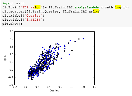
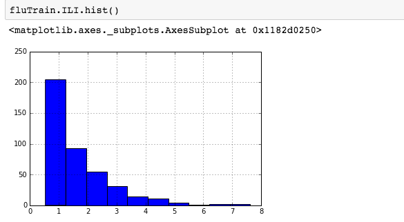     suggesting the distribution is right skewed- ie most of the ILI values are small with a relatively large number of values being large. However a plot of the natural log of ILI vs Queries shows that their probably is a positive linear relation between ln(ILI) and Queries.

:  

Time Series Model: 

In Google Flu trends problem set, initially we attempt to model log(ILI) as a function of Queries:

but since the observations in this dataset are consecutive weekly measurements of the dependent and independent variable, it can be thought of as a time-series.  Often Statistical models can be improved by predicting current value of the dependent variable using past values. Since most the ILI data has a 1-2 week lag- we need will use data from 2 weeks ago and earlier. Well how many such data points are there -ie  many values are missing from this variable ?  Calculating lag:

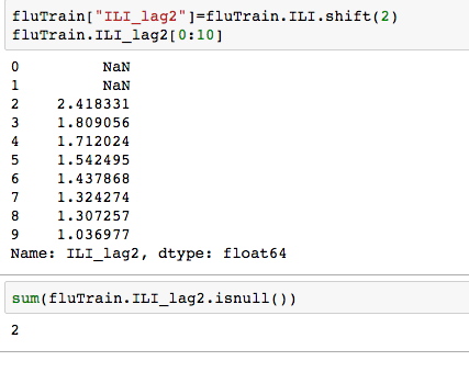
Plotting the log of ILI_lag2 vs log IL1, we notice a strong linear relationship.

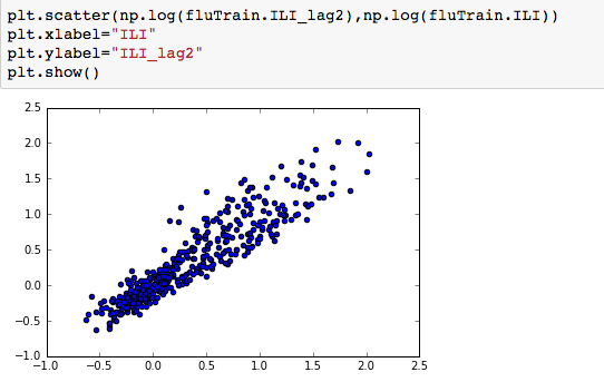
We can thus use both Queries and log(ILI_lag2), to predict log(ILI) and this significantly improves the model- increasing the R2 from 0.70 to 0.90. and the RMSE on the test set also reduces significantly.

Running regression models using all numerical variables is interesting, but one can use Categorical variables as well in the model!

Encoding Categorical Variables : To include categorical features in a Linear regression model, we would need to convert the categories into integers. In python, this functionality is available in DictVectorizer from scikit-learn, or “get_dummies()” function. One Hot encoder is another option. The difference is as follows:

1. OneHotEncoder takes as input categorical values encoded as integers – you can get them from LabelEncoder.
2. DictVectorizer expects data as a list of dictionaries, where each dictionary is a data row with column names as keys

One can also use Patsy (another python library) or get_dummies() see- Reading test scores. If you are using  statsmodels, you could also use the  C() function (see Forecasting Elantra sales)

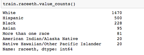
Pandas ‘get_dummies’ is I think the easiest option. For example, in the Reading Test Scores Assignment, we  wish to use the categorical variable ‘Race’ which has the following values:

Using get_dummies:

But we need only k-1 = 5 dummy variables for  the Race categorical variable. The reason is if we were to make k dummies for any of your variables, we would have a collinearity. One  can think of the k-1 dummies as being contrasts between the effects of their corresponding levels, and the level whose dummy is left out. Usually the most frequent category is is used as the reference level.

Other great Resources:

• assumptions of linear regression.
• An Introduction to Statistical Learning
• simple linear regression and multiple linear regression.
• quick reference guide