Tag Archives: LDA

Hierarchical clustering – what does that even mean, in terms of my topic models?

(continued from Topic Modeling …)

So great, I ran LDA, got 150 topics, and now I wanted to see if one could group these topics together using clustering. How can one go about doing that? Well as part of the process, LDA basically creates a “vocabulary” consisting of all the words from the corpus. As this number may get unmanageably large, as part of the LDA preprocessing, one  removes words like a, an, the, if where (also called stopwords) as may not really help decide whether a document belongs to a certain topic or not. There are other text learning tricks like stemming and lemmatization that I thought were not necessarily useful this context, but can often be useful and help control the size of the vocabulary. Well the vocabulary from my run contained ~650,000 words and mallet  allows you to output, for every topic, the word counts for all these words! So now you have a representation of all the topics in terms of their “word vectors”! And one can use this word vector to calculate “distances” between topics.

So after some data wrangling and manipulation, I had the topics represented in a numerical matrix, and ran the clustering algorithm on them. There are many variations of hierarchical clustering algorithms, and I tried most them to see which one seemed the best. I finally went with average linkage and shown below are some of the branches that clustered together. Instead of showing, topic numbers as leaves, we are displaying the word cloud represented by the topic at that leaf:

Figure on the left could be thought to represent a neuroimaging cluster and the figure to the right could be thought to represent disease and trauma. These images are courtesy  Natalie Tellis- Thanks Natalie!!

neuroscience

disease_trauma research

Unfortunately, we had to do a significant amount of manual curation, as some of the clusters didn’t make sense the way we humanly think of these topics …though algorithmically speaking they probably were “sisters”.  We wound up having twenty supertopics or umbrella topics  which contained the topics that LDA had produced. The naming of topics was done manually and was strongly influenced by the top most words for that topic.  

For example the supertopic called “Genetics and Genomics”, and “cellBiology”  have the following subtopics:

tpc_subtpc_slide

Topic Modeling- continued…

So continuing with Topic Modeling…(see earlier post)

Well -the time had come to confront pubmed- the real data I was going to work with. To start with I decided to only use 2013 pubmed data to see if I could run LDA on it and get out meaningful topics. Well, what do I mean by pubmed data: As I explained earlier, pubmed is a repository containing almost *all* research literature pertaining to the biomedical field. Since it is maintained and funded by NIH, we as the tax payers can access or scrape data from it! The only caveat is that only a small subset of papers have the entire text, and they are housed in what is called Pubmed CentralFor the rest of the data we can access things like: title, abstract, keywords (if any), journal name, journal ISSN number, date of publication, date created, date last modified etc.

In preparing the text corpus for LDA, we decided to use only the title and abstract. So, for all the records published in 2013, I parsed out the title and abstract, and created a text corpus containing one record per line, with the pmid as the record identifier. It looked something like this:

The real challenge for LDA is figuring out how many topics or categories should you try to divide the corpus into. I played around with K=10,12,14…500.  It seemed to me that the larger the K, more “fine” grained my topics: but was there an “intrinsic” number of topics that pubmed was naturally divided into… but remember each paper or record has a non zero probability of belonging to every topic- its a mixture of topics. So we could think about each “topic” as a dimension, and each paper belonging to this K dimensional space. And intuitively I felt that we went with a really large K, we would get a really high resolution among topics (which  we could think of as subtopics)- and then if we ran hierarchical clustering on this large number of topics, we could “cluster” similar topics thus naturally forming the “super topics”. I was excited. The challenge was that as K grew large, so did my job of trying to make sure that indeed all the topics made sense.

The road was quite bumpy. For example, I initially included keywords along with the abstracts in the text corpus, but found that keywords were present only in about 30% of the papers!. Earlier I had thought that perhaps the keywords could make up the main “vocabulary” of the corpus and be used to describe it- but that did not seem to be the case. Furthermore, in many cases the keyword tended to be names of particular chemical compounds which could not really “describe” the paper. I also had to check and see if the topics made sense. One way to do this was, for a  given value of K, to look at the top 20 words of the topic and see if the words seem to point to a coherent topic. If so, then pull out all the papers that had a high probability of being assigned to that topic (say >0.7) and look at them.

To see how good my topic modeling really was, I decided to ask the inverse question: if I picked specific journals ( that I know were represented in the corpus) , pulled out all the papers from journals, and summed the topic probabilities of those papers, I would get a “topic distribution” for that set of journals. What did that look like? I decided to pick specialized journals like “Cancer”, “Oncology Letters”, “Oncoimmunology”, OncoTargets (which could represent a specific topic “cancer”) and The Science of the total environment, Environmental pollution, Environmental toxicology and pharmacology, and  Environmental toxicology and chemistry which could be thought to represent “environmental science”.

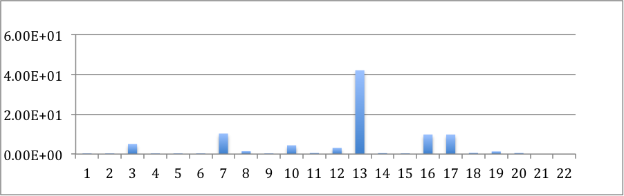
Figure A below is the topic distribution for the journal “Cancer“. As you can see topic 13 has avery high representation. Figure B shows the topic distribution if papers published in Oncology Letters”, “Oncoimmunology” and “OncoTargets” are included. You can see, topic 13 continues to have a high representation, but representation for topic 3 has also gone up. 

Figure A .  Cancer1  

Figure B.  Cancer2

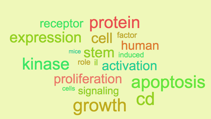
So what are topic 13 and topic 3? Here are word cloud representations of their top most words:

Screen Shot 2014-10-02 at 10.15.51 PM  topic 13      Screen Shot 2014-10-02 at 10.16.45 PM   topic 3


These word clouds make sense given that the journals were Cancer, Oncology letters etc; the high representation of topic 13 is very heartening.

 Figure C. below is the topic distributions for the journal The Science of the total environment, and Figure D is the topic distribution for papers from journals The Science of the total environment, Environmental pollution, Environmental toxicology and pharmacology, Environmental toxicology and chemistry. Topics 4 and 2 are the most dominant.

  Figure C.  env1

Figure D. env2 

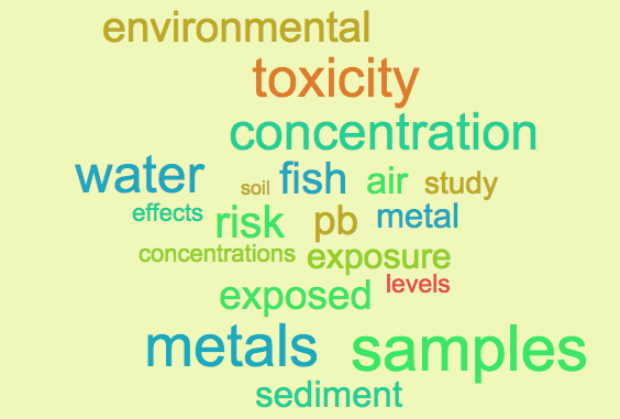
And here is  the word clouds for topics 4:   Screen Shot 2014-10-02 at 10.34.35 PM

As you can see it doesn’t conjure up the topic “environmental science”. But then the question is, is the value of K too small to “resolve” the topic “environmental science”? we can look at what happens when K is larger. Figure E shows the distribution of the same papers as included in Figure D, but assuming that we have run lda with K=50 on them.

env3

As you can see, it topic 15 that dominates. Here is the word cloud for topic 15 and this looks much more like environmental science!!

Screen Shot 2014-10-02 at 10.47.05 PM

So what value of K( ie number of topics) should we go with?                                                                       After conducting many experiments like these, we decided to go with K=150. Yes, K=150 is a large number but the thinking was that we could run the hierarchical clustering  on the topics themselves and see if how they clustered together and then each cluster could be considered a “supertopic”  or category and the topics that were contained in it,  would be the finer classification.  On the other hand 150 was manageable , in case we needed to perform some manual curation.

Topic Modeling: LDA… LSI.. Oh My!

As I explored the topics in text mining, and machine learning, I learned that there is an area of research called Topic Modelling. A  topic model is a type of statistical model for discovering the abstract “topics” that occur in a collection of documents. A topic modeling tool takes a collection of unstructured texts, and looks for patterns in the use of words – and a  “topic” consists of a cluster of words that frequently occur together. Using contextual clues, topic models can connect words with similar meanings and distinguish between uses of words with multiple meanings. Note that the algorithm has no knowledge of the semantic meaning of the words. Its an exercise in statistical probability. As a result every piece of text has some non zero probability of belonging to every topic. Naively, you say text A belongs to topic XX if it has a high probability of belonging to XX. Conversely, a peice of text could belong to multiple topics. Pretty cool!

I couldn’t wait to get my hand dirty. In their first incarnation(~1998), topic models were called Latent Semantic Indexing (LSI). Today, the most popularly used topic model is    Latent Dirichlet allocation (LDA). You can find links to lots more resources on David Blei’s  (one of the best known experts in topic modeling) site. I also learned a lot from some digital humanities sites like the programming historian and topic modelling for humanists. (At the time of writing this blog (which is ~ten months after I was learning about this), LDA has become the new rage and there are a lot more implementations of it with easy interfaces.)

I played with a bunch of freely available LDA implementations including Gensim, mallet, and lda-c. I found mallet to be the easiest to use and give me the most sensible results.

For my experiment, I went into pubmed, and searched for documents with the following terms in the abstract or title. I tried to pick terms that (I thought) were distinct. My hypothesis was that if I pulled out the abstracts and titles of the documenst pulled out in thsi way, combined them into a random ordered list, and fed it to LDA, and specified the number of “topics” I wanted; I could get back my classified list.

          terms in abstract or title                                              # of documents   

  1.  male breast cancer[Title/Abstract]                                            811
  2.  gluten free diet [Title/Abstract]                                                2790
  3. childhood schizophrenia[Title/Abstract]                                   1683
  4.  microfluidics[Title/Abstract]                                                     2279
  5.  high protein diet [Title/Abstract]                                              1340
  6.  malaria[Title/Abstract]) AND india[Title/Abstract]                    1178
  7. chromatin associated[Title/Abstract]                                        1138
  8. juvenile diabetes[Title/Abstract]                                                  621
  9. typhoid fever [Title/Abstract]                                                     2414
  10. bioethics                                                                                    2818

The results were quite interesting.  Here are the top 20 words of the topics that were returned:

0        microfluidics microfluidic cell chemistry methods instrumentation analysis techniques based cells flow detection analytical high chip surface systems system devices

1        typhoid fever salmonella typhi bacterial patients drug immunology humans blood vaccines infections diagnosis infection vaccine therapy test treatment strains

2        schizophrenia disorders childhood child diagnosis disorder children humans adult studies risk onset adolescent patients age psychology male factors female

3        malaria india epidemiology health falciparum control diseases population plasmodium disease humans cases countries vivax study drug species incidence water

4        proteins dna chromatin genetics protein metabolism cells cell gene expression binding sequence nuclear transcription genes histone rna molecular genetic

5        bioethics ethics health research medical care humans ethical human issues patient social public professional moral approach life medicine clinical

6        protein diet high rats metabolism dietary blood effects fed animals low administration weight proteins dosage increased body intake activity

7       breast cancer male neoplasms aged brca genetics patients female risk humans genetic carcinoma disease mutations cases factors mutation analysis

8        diabetes complications patients humans disease blood mellitus type etiology female diseases diagnosis male insulin adult juvenile patient child therapy

9        disease celiac gluten patients diet free coeliac cd immunology humans intestinal diagnosis antibodies adult aged blood female child children

Pretty cool eh? The top words seem to indicate that the topics were pretty well categorized. But how well were the documents really classified?  To explore this further, I took all the documents that had an original topic id of say “cancer”, and plotted  the maximum probability predicted for that document. The color indicates the topic predicted by that probability. For example: the plots  below shows all the documents that were originally identified as cancer and chromatin.

docs identified as cancer topics       train_chromatin_tpids

All the dots in the plot represent papers that were originally selected to be that topic- so the true positives. The color of the dot, represents which topic the algorithm thinks the paper belongs to.  Comparing witht the legend,  the fact that majority of the dots in the chromatin plot are peach and in the cancer plot are olive green suggest a pretty high accuracy rate.  Infact :

# of  incorrectly classified cancer docs=16          out of  614       ~2.6%      # of  incorrectly classified chromatin docs=27        out of 876        ~3.0%

Unfortunately, things don’t look so good for all the topics . Here are the plots for Malaria and Typhoid:

train_typhoid_tpidstrain_malaria_tpids

As you can see, the accuracy here is significantly less:

# of  incorrectly classified malaria docs=166      out of 853         ~19.46%  # of  incorrectly classified typhoid docs=734     out of 1841     ~39.87%

Here are the numbers for the rest of the topics:                                                 # of  incorrectly classified gluten docs=279         out of 2094     ~ 13.3% # of  incorrectly classified schizophrenia docs=61    out of 1327 ~4.6% # of  incorrectly classified southbeach docs=94    out of 1027      ~9.1   #  of  incorrectly classified microfluidics docs=67  out of 1342   ~4.9%  # of  incorrectly classified diabetes docs=127        out of 489     ~ 25.9%  # of  incorrectly classified bioethics docs=69        out of 2166    ~3.18%

So, error in prediction 1640 /12629 =~12.98%. While this is a good start; it would be worth exploring what one could do to bring the error rate lower.